Diffraction Modelling

Using a numerical approximation of the Fourier Transform, we predict the resulting diffraction patterns produced from optical diffraction experiements with various shaped 2D sources in matrix representation.

Background

Optical signals are rarely monochromatic but rather a superposition of characteristic frequencies. These can be expressed as a Fourier Series of sine and cosine functions through the Fourier Series in 2D,

\[F\left(u,v\right)=\int_{-\infty}^{\infty}\int_{-\infty}^{\infty}{f\left(x,y\right)e^{-2\pi i(xu+yv)}}dxdy\]

This can be numerically discretized with the following compound sum,

\[F\left(u,v\right)=\frac{1}{4NM}\sum_{x=-N}^{N-1}\sum_{x=-M}^{M-1}\left(f\left(x,y\right)e^{-\pi i\left(\frac{xu}{N}+\frac{yv}{M}\right)}\right)\]

Sample Output

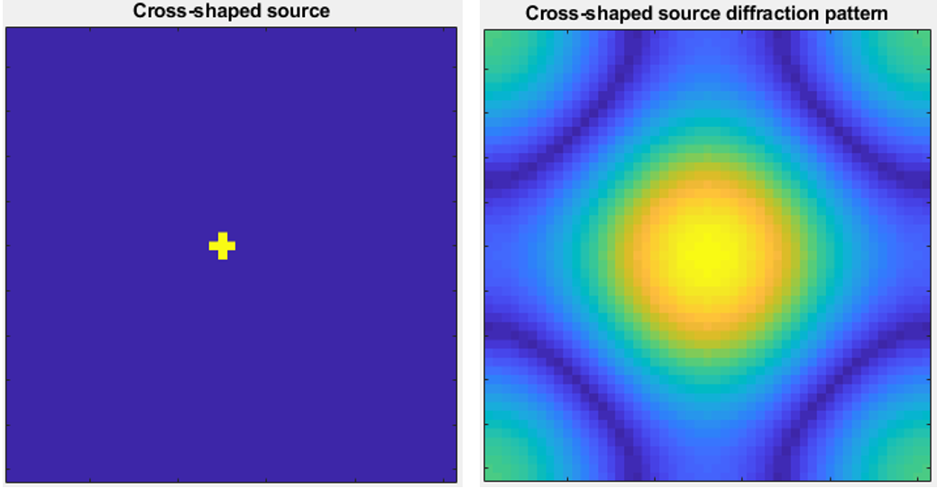
For a cross-shaped source, we see the expected output matrix displaying regular light diffraction through an aperture.

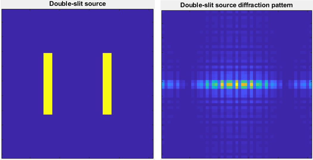
For a double slit, we reproduce the same characteristic fringe interference as seen in Young’s Experiment, now in 2D.

This application of the Discrete Fourier Transform demonstrates the effectiveness of numerical modelling in quickly predicting experimental outcomes in optical physics.

The Discrete Fourier Transform is implimented in matrix representation with MATLAB and the following nested loop:

for a = 1:2*N+1 %Iterate over output array rows, index a 
    v = a-(N+1); %Convert output array row index to coordinates in v space
    for b = 1:2*M+1 %Iterate over output array cols, index b 
        u = b-(M+1); %Convert output array col index to coordinates in u space
        for c = 1:2*N+1 %Iterate over input array row elements, index b
            y = c-(N+1); %Convert input array index to coordinates in y space
            for d = 1:2*M+1 %Iterate over input vector col elements, index b
                x = d-(M+1); %Convert input array index to coordinates in x space
                Y(a,b)= Y(a,b) + X(c,d)*exp(-i*pi*((u*x/M) +(v*y/N))); %Compute double summation for output vector elements

See source code on my GitHub for further details.